D. M. Pan National Real Estate Company’s Housing Price Prediction Model
Introduction
This report was commissioned by the CEO of D. M. Pan National Real Estate. The purpose of this report is to provide a benchmark price for square foot of real estate based on the statistical analysis of the real estate prices in the US in 2019. The central question this report aims at answering is, ‘what benchmark price should D. M. Pan National Real Estate to list houses based on square footage. In order to answer this question, the report uses a dataset of 50 randomly selected houses in different parts of the US to create a linear regression model that would provide an equation for pricing the houses.
We will write acustom essay on your topictailored to your instructions!
188experts online
Creating a linear regression model is most appropriate when there is a strong correlation between a predictor and an outcome variable. A scatterplot for such a relationship looks a collection of dots scattered around a straight line that is either ascending or descending. A predictor variable is an independent variable that affects the response variable if manipulated. A response variable is dependent to some extent on the predictor variable. Since the square footage is assumed to affect the price of the real estate positively, the price was selected to be a response variable and the square footage was selected to be a predictor variable.
Data Collection
The data for the analysis was collected from a dataset of 1,000 entries that included prices, square footage, and prices per square foot of real estate objects all over the US with their location in terms region, state, and county. A random sample of 50 entries was selected using Microsoft Excel by creating a new column with a random number, sorting the list of entries according to the random number, and selecting first 50 entries. The predictor variable (x-axis) was square footage of the house, while the responses variable (y-axis) was the price of the house. The data is visualized in Figure 1 below using a scatterplot.
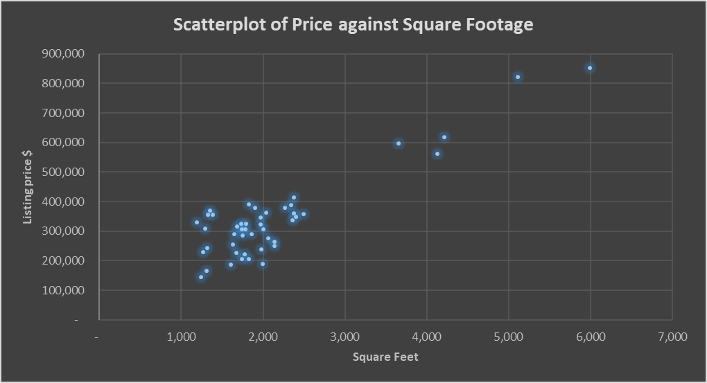
Figure 1. Scatterplot of listing price against square footage
On-time delivery!
Get your 100% customized paperdone in as little as 1 hour
The scatterplot demonstrates that the dots on the graph are clustered along an ascending straight line, which is a sign of a linear correlation. Thus, using a linear regression model for predicting the listing price is appropriate.
Data Analysis
Before conducting regression analysis, descriptive analysis of the variables was conducting using summary statistics and histograms. The histograms for square footage and listing price of the sample are provided in Figures 2 and 3 correspondingly. Summary statistics of the sample are provided in Table 1 below.
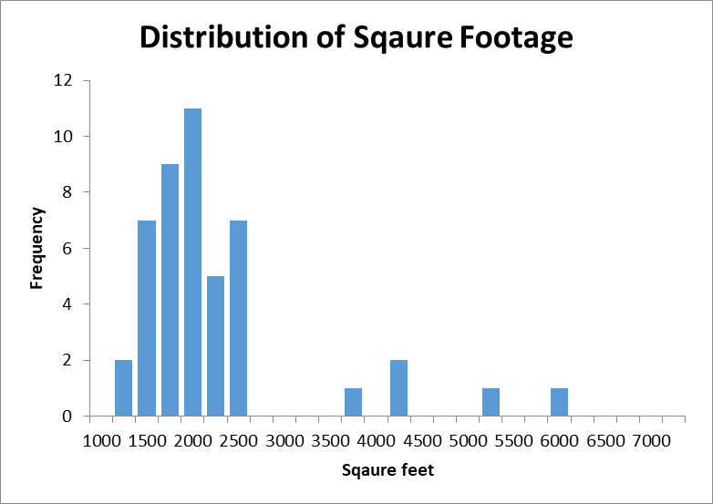
Figure 2. Distribution of sample square footage of the houses
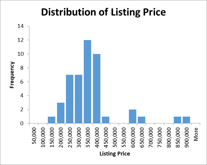
Figure 3. Distribution of the sample listing price
Deadline panic?
We're here to rescue and writea custom academic paperin just 1 hour!
Table 1. Descriptive sample statistics
| Square Feet | Listing Price | |
| Mean | 2,122 | 339,450 |
| Median | 1,843 | 319,900 |
| Standard Deviation | 985 | 145,568 |
The analysis demonstrates that the distribution of the square footage wand the listing prices were close to normal with a positive skew, as the values were clustered on the left side of the distribution. The distributions also appear to be highly leptokurtic, as they are concentrated around the mean. There are also significant gaps and outliers on the right side of the distributions. The presence of outliers may have affected them mean value. The average square footage of the houses was 2,122 with a standard deviation of 985 and a median value of 1,843. The average listing