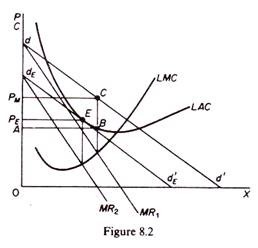
 The firm, being in equilibrium (at C), does not have any incentive to change its price. The abnormal profits will, however, attract new competitors into the market. The result of new entry is a downward shift of the demand curve dd’, since the market is shared by a larger number of sellers. Assuming that the cost curves will not shift as entry occurs, each shift to the left of the dd’ curve will be followed by a price adjustment as the firm reaches a new equilibrium position, equating the new marginal revenue (on the shifted MR curve) to its marginal cost.
The process will continue until the demand is tangent to the average-cost curve, and the excess profits are wiped out. In the final equilibrium of the firm the price will be PE and the ultimate demand curve dEd’E. This is an equilibrium position, since price is equal to the average cost. There will be no further entry into the industry, since profits are just normal. The equilibrium is stable, because any firm will lose by either raising or lowering the price PE.
Model 2: equilibrium with price competition:
In this model it is assumed that the number of firms in the industry is that which is compatible with long-run equilibrium, so that neither entry nor exit will take place. But the ruling price in the short run is assumed to be higher than the equilibrium one.
ADVERTISEMENTS:
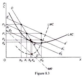
The analysis of this case is done by the introduction of a second demand curve, labelled DD’ in figure 8.3, which shows the actual sales of the firm at each price after accounting for the adjustments of the prices of other firms in the group. DD’ is sometimes called actual-sales curve or share-of-the-market curve, since it incorporates the effects of actions of competitors to the price changes by the firm. The DD’ curve shows the full effect upon the sales of the firm which results from any change in the price that it charges.
 DD’ is thus the locus of points of shifting dd’ curves as competitors, acting simultaneously, change their price. It should be clear that the change in the price does not take place as a deliberate reaction to other firms’ reductions, but as an independent action aiming at the profit maximization of each firm acting independently of the others.
The DD’ curve shows a constant share of the market, and, as such, it has the same elasticity as the market demand at any one price. Clearly the DD’ curve is steeper than dd’, because the actual sales from a reduction in P are smaller than expected on the basis of dd’ as all firms reduce their price and expand their own sales simultaneously.
ADVERTISEMENTS:
A movement along DD’ shows changes in the actual sales of existing firms as all of them adjust their price simultaneously and identically, with their share remaining constant. A shift in the DD’ is caused by entry of new firms or exit of existing firms from the ‘industry’ and shows a decline or an increase in the share of the firm.
Assume that the firm is at the non-equilibrium position defined by price P0 and quantity X0. The firm, in an attempt to maximize profits, lowers the price at P1 expecting to sell, on the basis of its individual demand curve, quantity X’0. This level of sales is not actually realised, because all other firms, faced by the same demand and cost conditions, have the incentive to act in the same way simultaneously. Each one attempts to maximise its own profit, ignoring the reactions of competitors, on the assumption that the effect on the demand of other firms in the group is negligible.
Thus all firms, acting independently, reduce their price simultaneously to P1. As a result the dd’ curve shifts downwards (d1d’1) and firm A, instead of selling the expected quantity X’0, sells actually a smaller quantity X1 on the shifted-demand curve d1d’1 and along the share curve DD’. One might think that the firm would learn to anticipate similar shifts in the future if it decided to reduce its price.
However, according to the model, the firm suffers from myopia and does not learn from past experience. It continues to behave on the assumption that its new demand (d1d’1) will not shift further, because the effect of its own decisions on other sellers’ demand would be negligible. Thus the firm lowers its price again in an attempt to reach equilibrium, but instead of the expected sales X’0 the firm achieves actual sales X2, because all other firms act identically, though independently.
The process stops when the dd’ curve has shifted so far to the left as to be tangent to the LAC curve. Equilibrium is determined by the tangency of dd’ and the LAC curve (point e in figure 8.3). Any further reduction in price will not be attempted since the average cost would not be covered.
In summary, the individual demand curve dd’ explains why each firm is led to reduce its price. The DD’ curve shows the firm’s actual sales as the general downward cut in price takes place. The dd’ curve slides downwards along the DD’ curve as prices are lowered, and the adjustment process comes to a stop when the dd’ is tangent to the LAC curve. At the point of tangency the DD’ curve cuts the dd’ curve. Obviously it will pay no one firm to cut the price beyond that point, because its costs of producing the larger output would exceed the price at which this output could be sold in the market.
Model 3: price competition and free entry:
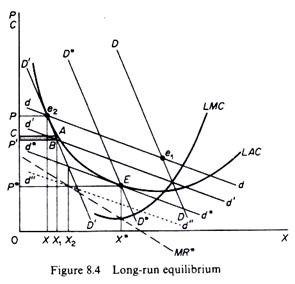
Chamberlin suggests that in actual life equilibrium is achieved both by price adjustments of the existing firms and by new entry. Price adjustments are shown along the dd’ curve while entry (and exit) cause shifts in the DD’ curve. Equilibrium is stable if the dd’ curve is tangent to the AC curve and expected sales are equal to actual sales, that is, if the DD’ curve cuts the dd’ curve at the point of its tangency to the AC curve. Let us examine how the equilibrium tangency solution is reached (figure 8.4).
 It is assumed that profits at point e1 are abnormal. New firms are attracted until DD shifts to D’D’. One might think that e2 is a long-run equilibrium (with price P and output X) since only normal profits are earned. However, this is not the case, because each entrepreneur thinks that dd is his demand curve, and consequently he believes that if he reduced his price his sales would expand along dd and profits would increase. But each firm has exactly the same incentive and all firms reduce their price.
ADVERTISEMENTS:
As price is reduced by all firms dd slides down D’D’ and each firm realises a loss instead of positive abnormal profits. For example, at position d’d’ the firm has reduced its price to P’ but, as all firms act similarly, X1 is produced with a total loss equal to the shaded area ABP’C.
However, the firm acts on the ‘myopia curve’ d’d’ and so long as this lies above the LAC, it believes that it can obtain positive profits by cutting its price. The loss increases still further as dd slides further down along D’D’. One might think that the process would stop when dd becomes tangent to the LAC. This would be so if the firm could produce X.
However, there are too many firms in the industry and the share of the firm is only X2 (on D’D’). The firm still on the ‘myopia assumption’ believes that it can reach X if it reduces price to P. However, all firms do the same and dd falls below the LAC with ever-increasing losses.
ADVERTISEMENTS:
The financially weakest firms will eventually leave the industry first, so that the surviving firms will have a larger share. D’D’ moves to the right together with dd. Exit will continue until dd becomes tangent to the AC curve and DD cuts dd at the point of the tangency, E. Equilibrium is then stable at point E with normal profits earned by all firms and no entry or exit taking place. The equilibrium price P is unique and each firm has a share equal to 0X.